MatheAss 9.0 - Analysis

p(x) = x5 - 9·x4 - 82/9·x3 + 82·x2 + x - 9
       = (1/9)·(9·x5 - 81·x4 - 82·x3 + 738·x2 + 9·x - 81)
       = (1/9)·(3·x - 1)·(3·x + 1)·(x - 9)·(x - 3)·(x + 3)

Rational zeros: 1/3, -1/3, 9, 3, -3

Transforming Polynomials (New in Version 9.0)

A polynomial function ƒ(x) can be shifted or stretched in the x direction and y direction.

ƒ(x) = - 1/4·x4 + 2·x3 - 16·x + 21

Shifted by dx = -2, dy = 0                                           

ƒ(x + 2) = - 1/4 ·x4 + 6 ·x2 + 1

Polynomials GCD and LCM (new in version 9.0 from February 2021)

The program calculates the greatest common divisor (GCD) and the least common multiple (LCM) of two polynomials p₁(x) and p₂(x).

p1(x) =  4·x6 - 2·x5 - 6·x4- 18·x3 - 2·x2 + 24·x + 8
p2(x) =  10·x4- 14·x3 - 22·x2 + 14·x + 12

GCD(p1,p2) =  x2 - x - 2
LCM(p1,p2) =  40·x8 - 36·x7 - 76·x6 - 144·x5 + 88·x4+ 356·x3 - 4·x2 - 176·x - 48

Function Plotter

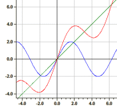
Up to ten functions can be drawn simultaneously in a coordinate system. Links or derivatives of already defined functions are also permitted.

If   ƒ1(x) = sin(x)  and  ƒ2(x) = 3*sqrt(x), then 

ƒ3(x) = 2*y1^2-y2   substitudes    ƒ3(x) = 2*sin(x)^2-3*sqrt(x)
ƒ4(x) = f2(y1)         substitudes     ƒ4(x) = 3*sqrt(sin(x))
ƒ5(x) = y2'              substitudes     ƒ5(x) = 3/(2*sqrt(x))

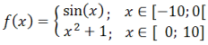
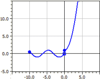
Piecewise Functions

A function defined in sections is drawn, which is given by up to nine subfunctions. For each of the subfunctions, the definition area, the type of interval, and the color are entered. It is also possible to determine whether the boundary points are drawn or not.

Example:

Parameter curves

With this program, curves can be drawn that are not given by an explicit function term, but by two functions for horizontal and vertical deflection.

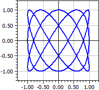
Des figures de Lissajou sont obtenus lorsque deux tensions alternatives de fréquences différentes sont appliquées à un oscilloscope.

Lissajou figures are obtained when two a-c voltages with different frequencies are applied to an oscilloscope.

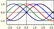
Family of Curves

The program draws the graphs of any function that contains a blade parameter k. The values for k can be listed or determined by initial value, end value and step size.

Calculus of Polynomial Functions (New in Version 9.0)

The program performs the curve discussion for a polynomial function. That is, the derivatives and the root function (antiderivative) are determined, the function is examined for rational zeros, extremes, turning points and symmetry.

Function:
¯¯¯¯¯¯¯¯
ƒ(x) = 3·x4 - 82/3·x2 + 3
       = 1/3·(9·x4 - 82·x2 + 9)
       = 1/3·(3·x - 1)·(3·x + 1)·(x - 3)·(x + 3)

Derivations:
¯¯¯¯¯¯¯¯¯¯
ƒ'(x)  = 12·x3 - 164/3·x
ƒ"(x)  = 36·x2 - 164/3
ƒ'"(x) = 72·x

Antiderivative:
¯¯¯¯¯¯¯¯¯¯¯
F(x) = 3/5·x5 - 82/9·x3 + 3·x + c

  .
  .
  .

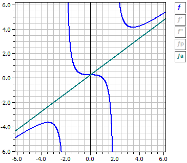
Calculus of Rational Functions (New in Version 9.0)

The program performs the curve discussion for a rational function. That is, the derivatives, the definition gaps and the continuous continuation are determined. The function is examined for zeros, extrema, turning points, and behavior for |x|→ ∞.

Function :
¯¯¯¯¯¯¯¯
             3·x3 + x2 - 4        (x - 1)·(3·x2 + 4·x + 4)  
ƒ(x) = —————— = ———————————
                4·x2 - 16               4·(x - 2)·(x + 2)       

Singularities:
¯¯¯¯¯¯¯¯¯¯¯
x = 2  Pole with change of sign
x =-2  Pole with change of sign

Derivatives:
¯¯¯¯¯¯¯¯¯¯
               3·(x4 - 12·x2)            3·(x2·(x2 - 12))   
ƒ'(x) = ———————— = ————————
            4·(x4 - 8·x2 + 16)       4·(x - 2)2·(x + 2)2 

                      6·(x3 + 12·x)               6·(x·(x2 + 12))  
ƒ"(x) = ——————————— = ———————
              x6 - 12·x4 + 48·x2 - 64       (x - 2)3·(x + 2)3 
  .
  .
  .

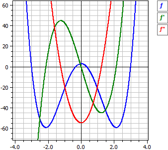
Calculus of arbitrary Functions

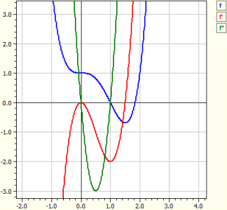
The program performs the curve discussion for any function. That is, the derivatives are determined, the function is examined for zeros, extrema and turning points, the graphs of ƒ, ƒ' and ƒ" are drawn, and a table of values is output.

Function:
‾‾‾‾‾‾‾‾‾‾‾‾
  ƒ(x) = x^4-2*x^3+1
  Examination in the range from -10  to  10

Derivations:
‾‾‾‾‾‾‾‾‾‾‾‾‾‾‾
  ƒ'(x) = 4*x^3-6*x^2
  ƒ"(x) = 12*x^2-12*x

Zeros:
‾‾‾‾‾‾‾‾
  N1(1|0)                     m = - 2
  N2(1,83929|0)          m = + 4,5912

Extremes:
‾‾‾‾‾‾‾‾‾‾‾‾‾
  T1(1,5|-0,6875)        m = 0

Pts of inflection:
‾‾‾‾‾‾‾‾‾‾‾‾‾‾‾‾‾‾‾‾‾
  W1(0|1)                   m = + 0
  W2(1|0)                   m = - 2

Newton Iteration

Newton iteration is an approximation method for calculating a zero of ƒ(x). If you enter a starting value x₀ that is close enough to the desired zero, the next approximation is the intersection of the tangent to the graph of f in the point P(x₀ / ƒ(x₀)).

  ƒ(x) = x-cos(x)

                 x                       ƒ(x)                  ƒ'(x) 
   ————————   ——————   ——————   
   x0 = 1
   x1 = 0,75036387     0,45969769       1,841471
   x2 = 0,73911289     0,018923074     1,681905
   x3 = 0,73908513     0,00004646       1,6736325
   x4 = 0,73908513     0,00000000       1,673612

Integral Calculus (from February 2021 with arc lengths)

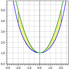
The oriented and absolute contents of the surface between two function curves are calculated at a desired interval [a; b].
In addition the twisting moments for rotation, the bodies of revolution and the arc lengths in the interval.

  ƒ1(x) = cosh(x)
  ƒ2(x) = x^2+1

  Limits of integration from  -2  to  2

  Oriented content  :  A1 = -2,07961
  Absolute content  :  A2 = 2,07961

  Arc lengths          :  L1[a;b] = 7,254      L2[a,b] = 9,294 

Series Development

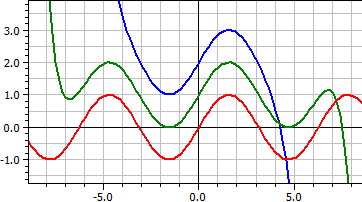
A function given as a series is drawn, whereby the series developments for different parameter ranges can be compared and moved in the y-direction for better differentiation.

The first 16 members of the Taylor series
for the sine function. .

ƒ(x,k) = x^(2*k-1)/fac(2*k-1)*(-1)^(k+1) ,   
k = 4, 8 und 16

Surface Functions

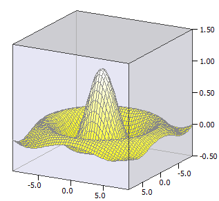
A surface function ƒ(x,y), i.e. the three-dimensional diagram of a function with two variables, is drawn.

eng.matheass.eu